 |
G+Smo
25.01.0
Geometry + Simulation Modules
|
 |
G+Smo
25.01.0
Geometry + Simulation Modules
|
This tutorial provides a basic motivation for truncated hierarchical B-splines (THB-splines) and a brief introduction to some basic features of gsTHBSplineBasis.
See also basis_example.cpp and bSplineBasis_example.cpp.
More details on the hierarchical splines can be found in adaptRefinementThb_example.cpp as well as in the Hierarchical splines module description.
Two simple examples are provided for illustrating the construction of a THB-spline basis. The formal definition is given only for the sake of completeness (see Formal definition), see the References for further details.
For illustration, consider a 1D-example.
We start with two sets of B-Spline basis functions of degree 2:
Level 0, the "coarse" ones, with knot vector \( s^0 = (0,\ 0,\ 0,\ 1/8,\ 2/8,\ ... 7/8,\ 1,\ 1,\ 1)\)
Level 1, the "fine" ones, with knot vector \( s^1 = (0,\ 0,\ 0,\ 1/16,\ 2/16,\ ... 15/16,\ 1,\ 1,\ 1)\)
These two bases are illustrated here (shown in different colours and thickness only for better visibility):


The parameter domain is referred to as \( \Omega^0 \). The green area in the pictures indicates \( \Omega^1 \subset \Omega^0 \), i.e., the area where we want finer basis functions.
A straightforward way of doing so: Take all fine functions \( \beta^1_j \) where \( \mathrm{supp} \beta^1_j \subset \Omega^1 \),

...and only those coarse functions \( \beta^0_i \) where \( \mathrm{supp} \beta^0_i \subset \Omega^0 \land \mathrm{supp} \beta^0_i \not \subset \Omega^1 \)

By taking the union of these two sets of functions, we obtain the hierarchical B-spline basis (HB-splines) of level 1:

With this basis, however, the partition-of-unity property is lost. Also, there can be large overlaps of the supports of the basis functions.
Instead of just using the coarse functions as they are, the coarse functions are truncated (see References at the bottom for details). This results in the THB-spline basis of level 1:

THB-splines again have the partition-of-unity property and support overlaps are reduced.
Note that HB-splines and THB-splines span the same function space.
Similar to the 1D-case above, consider a coarse and a fine mesh, as displayed on the left, and right, respectively. The corresponding tensor-product B-spline bases of degree 2 are displayed in the picture below. The green area again indicates the area where we want fine basis funcitons.
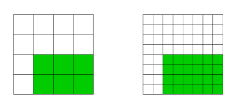
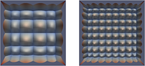
As in the 1D-case, we select
the coarse functions \( \beta^0_i \) where \( \mathrm{supp} \beta^0_i \subset \Omega^0 \land \mathrm{supp} \beta^0_i \not \subset \Omega^1 \), and we truncate them (displayed on the left)
and the fine functions \( \beta^1_j \) where \( \mathrm{supp} \beta^1_j \subset \Omega^1 \) (displayed on the right):
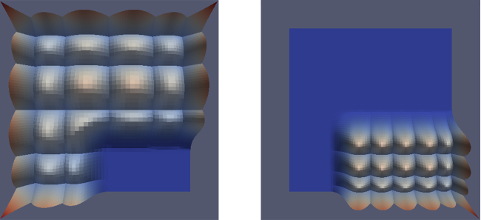
The union of these functions is the THB-spline basis:
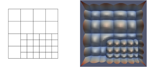
Just for the sake of completeness, a brief formal definition is provided, without going into any details. See References at the bottom for details
Let \( B^{\ell-1} \) denote the (tensor-product) B-spline basis of level \(\ell - 1 \). Let a function \( \tau \in \mathrm{span} B^{\ell-1} \) be represented in terms of \( B^{\ell} \) by \( \tau = \sum_{\beta^{\ell} \in B^{\ell} } c_\beta \beta^{\ell} \). The truncation of \( \tau \) is given by \( \mathrm{trunc}^{\ell} \tau = \sum_{\beta^{\ell} \in B^{\ell},\ \mathrm{supp} \beta^{\ell} \not \subseteq \Omega^{\ell} } c_\beta \beta^{\ell} \)
\( T^0 = B^0 \)
\( T^{\ell} = T_A^{\ell} \cup T_B^{\ell}\), where
\( \quad T_A^{\ell} = \{ \mathrm{trunc}^{\ell} \tau:\ \tau \in T^{\ell-1} \land \mathrm{supp} \tau \not \subseteq \Omega^{\ell} \} \)
\( \quad T_B^{\ell} = \{ \beta^\ell \in B^{\ell}:\ \mathrm{supp} \beta^\ell \subseteq \Omega^{\ell} \} \)
\( T = T^N \)
Remark: gsTHBSplineBasis and gsHBSplineBasis are derived from gsHTensorBasis
Constructor using a gsTensorBSplineBasis as argument.
Example for a THB-spline basis of degree 2:
<?xml version="1.0" encoding="UTF-8"?>
<xml>
 <Basis type="THBSplineBasis2" levels="6">
  <Basis type="TensorBSplineBasis2">
   <Basis type="BSplineBasis" index="0">
    <KnotVector degree="2">0 0 0 1 1 1 </KnotVector>
   </Basis>
   <Basis type="BSplineBasis" index="1">
    <KnotVector degree="2">0 0 0 1 1 1 </KnotVector>
   </Basis>
  </Basis>
 </Basis>
</xml>
The tensor-product B-spline basis in the "THBSplineBasis2" defines the basis of level 0.

See gsHTensorBasis::refineElements(). The argument is a std::vector<unsigned> containing a sequence of n*(1+2*d) unsigned. Each (1+2*d)-tuple contains the following information:
The green are marked in the 2D-example above has lower corner (2,0) and upper corner (8,4) in unique knot indices at level 1. We can refine this area as follows:
This method is the recommended one, since the corners of the refinement areas are specified by unsigned integers, which is numerically stable. Also, since the level is specified explicitly, double calls by mistake will not result in double refinement.
One can also specify different levels of refinement already in the xml-file, using the "box"-tag:
<?xml version="1.0" encoding="UTF-8"?>
<xml>
 <Basis type="THBSplineBasis2" levels="6">
  <Basis type="TensorBSplineBasis2">
   <Basis type="BSplineBasis" index="0">
    <KnotVector degree="2">0 0 0 1 1 1 </KnotVector>
   </Basis>
   <Basis type="BSplineBasis" index="1">
    <KnotVector degree="2">0 0 0 1 1 1 </KnotVector>
   </Basis>
  </Basis>
 <box level="1">2 0 8 4</box>
 </Basis>
</xml>
See gsHTensorBasis::refine(). The argument is a gsMatrix of size d x (2*n). Two columns represent the coordinates of the lower and the upper corner, respectively, of the area to be refined. In our example, the area to be refined can be written as
gsMatrix<real_t> boxM(2,2);
boxM(0,0) = 0.25;
boxM(1,0) = 0.0;

boxM(0,1) = 1.0;
boxM(1,1) = 0.5;

thb.refine( boxM );
This method refines all elements overlapping the specified box.
Warning!
This method does not specify which level should be refined to. If parts overlap, areas might get refined twice.
This refinement function uses numerical values, which could cause problems, especially when the coordinates coincide with knots.
Just like with the other bases. For example, displaying information via std::cout,
will return the following:
This basis is:
Truncated basis of dimension 2,
levels=2, size=54, tree_nodes=5).
Domain: [0 0]..[1 1].
Size per level: 30 24
The last line refers to the number of basis functions on the respective levels.
Other functions such as gsHTensorBasis::active_into(),
gsHTensorBasis::eval_into(),
gsHTensorBasis::deriv_into(), and also
gsHTensorBasis::uniformRefine() work as usual.
Example:
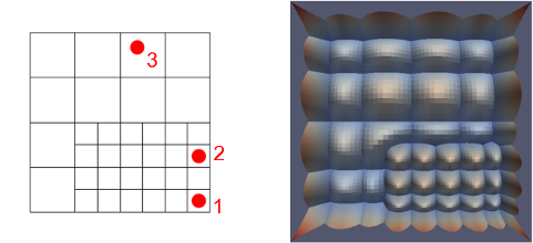
active functions:
 9  9 14
10 10 15
11 11 16
33 15 20
34 16 21
35 17 22
39 45 26
40 46 27
41 47 28
45 51  0
46 52  0
47 53  0
their values:
     0 0.0012 0.0144
     0 0.0204 0.0592
     0 0.0384 0.0064
0.0288 0.0004 0.1008
0.2016 0.0068 0.4144
0.1296 0.0128 0.0448
0.0448 0.0144 0.0648
0.3136 0.1008 0.2664
0.2016 0.0648 0.0288
0.0064 0.0592      0
0.0448 0.4144      0
0.0288 0.2664      0
Note:
The basis functions are numbered firstly by level (starting with level 0), and then by the tensor-index of the respective level (see Indexing / numbering of basis functions).
gsHTensorBasis::active_into() does not account for functions which are truncated to zero (i.e., it will return the same result for gsHBSplineBasis and gsTHBSplineBasis). Functions which are truncated to zero will be evaluated as (exactly) zero.
Some additional functions are specific to gsHTensorBasis.
The basis functions are numbered firstly by level (starting with level 0), and then by the tensor-index of the respective level.
The index in the numbering of the whole THB-spline basis (in our example, the numbering from 0 to 53), is referred to as global index or hierarchical index.
The index that a certain function has within the tensor-product B-spline basis of the respective level is referred to as flat tensor index ("flat" in the sense that no d-tupels are used, but the tensor-product basis functions already have a "single-digit" index).
To get the flat index and the level of a certain basis function, use gsHTensorBasis::flatTensorIndexOf() and gsHTensorBasis::levelOf().
will, in our example, print
transform indices
global/hier.index  ->  flat tensor index (on level)
27  ->  33  ( 0 )
28  ->  34  ( 0 )
29  ->  35  ( 0 )
30  ->  4  ( 1 )
31  ->  5  ( 1 )
32  ->  6  ( 1 )
33  ->  7  ( 1 )
34  ->  8  ( 1 )
35  ->  9  ( 1 )
To compute the global/hierarchical index from a given flat index and a given level, use gsHTensorBasis::flatTensorIndexToHierachicalIndex().
will, in our example, print
reverse index transformation
flat tensor index (on level)  ->  global/hier.index
33  ( 0 )  ->  27
34  ( 0 )  ->  28
35  ( 0 )  ->  29
4  ( 1 )  ->  30
5  ( 1 )  ->  31
6  ( 1 )  ->  32
7  ( 1 )  ->  33
8  ( 1 )  ->  34
9  ( 1 )  ->  35
gsHTensorBasis::getLevelUniqueSpanAtPoints() will tell you the levels of certain points, as well as the knot span containing these points:
In our example, this will return
levels:
1 1 0
lower corners:
7 7 2
0 2 3
These indices are given on the respective level.
The gsHTensorBasis are based on a gsHDomain. The tree-structure (see references at the bottom) can be accessed by the member function gsHTensorBasis::tree(). For example, this is how to take a look at the underlying tree-structure:
In our example, this will return
levels:
0
1
0
lower corners:
2 4
2 0
0 0
upper corners:
8 8
8 4
2 8
Note that these indices are given with respect to level gsHDomain::m_maxInsLevel.
Keep in mind that fine functions are only added, if the refined area contains the support of at least one fine basis function! If only a single cell/element is refined, no fine functions are added (for \( p > 1 \))! If necessary, extend the refinement area by a ring of cells around the refinement area.
Take the hierarchical mesh from above, where \( \Omega^1 \) is now coloured light green. Refining the dark green area to level 2 will NOT result in the mesh shown in the middle. Instead, in order to avoid L-shaped elements, and due to some requirements by the underlying tree, the mesh shown on the right will be generated (with additional refinement in the orange areas).

The hierarchical mesh and the corresponding THB-Spline basis:
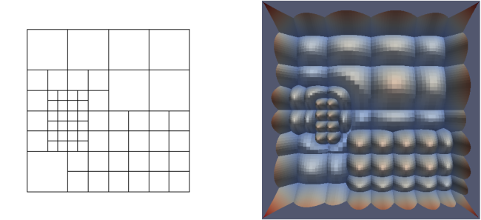
Applying this refinement to the basis and printing the basis...
...will return
after 2nd refinement, this basis is:
Truncated basis of dimension 2,
levels=3, size=70, tree_nodes=25).
Domain: [0 0]..[1 1].
Size per level: 30 32 8
This should be kept in mind when manually creating THB-spline geometries.
Assume you have given a certain spline geometry (curve, surface, volume,...) represented by tensor-product splines of level 0 with coefficients \( c^0_i \):
\[ G(\xi) = \sum_{ \beta^0_i \in B^0} c^0_i \beta^0_i(\xi) \]
The same geometry can be represented on level 1 with different coefficients \( c^1_j \):
\[ G(\xi) = \sum_{ \beta^1_j \in B^1} c^1_j \beta^1_j(\xi) \]
If an area \( \Omega^1 \subset \Omega^0 \) is refined to level 1, we obtain the THB-spline basis consisting of
The geometry \( G \) can be obtained exactly by taking the same coefficients \( c^0_j \) and \( c^1_j \) that were used on the respective levels:
\[ G(\xi) = \sum_{ \beta^0_i \in B^0,\ \mathrm{supp} \beta^0_i \not \subseteq \Omega^1} c^0_i\ \mathrm{trunc}^1 \beta^0_i(\xi) + \sum_{ \beta^1_j \in B^1,\ \mathrm{supp} \beta^1_j \subseteq \Omega^1} c^1_j \beta^1_j(\xi) \]
C. Giannelli, B. Jüttler, and H. Speleers. THB-splines: The truncated basis for hierarchical splines. Comput. Aided Geom. Design, 29(7):485-498, 2012. [Link] [Technical Report]
C. Giannelli, B. Jüttler, and H. Speleers. Strongly stable bases for adaptively refined multilevel spline spaces. Adv. Comp. Math., 40(2):459-490, 2014. [Link] [G+S Report No. 3]
C. Giannelli, B. Jüttler, S.K. Kleiss, A. Mantzaflaris, B. Simeon, J. Speh: THB-splines: An Effective Mathematical Technology for Adaptive Refinement in Geometric Design and Isogeometric Analysis. NFN Technical Report No. 30. [Link] [G+S Report No. 30]
G. Kiss, C. Giannelli, B. Jüttler: Algorithms and Data structures for truncated hierarchical B-splines. Mathematical Methods for Curves and Surfaces. Ed. by M. Floater et al. Vol. 8177. Lecture Notes in Computer Science. Springer, 2014, pp 304 - 323. [Link] [Technical Report]
Here is the full file examples/thbSplineBasis_example.cpp. Clicking on a function or class name will lead you to its reference documentation.