adaptRefinementThb_example.cpp

This tutorial, shows how to use some functions for adaptive refinement. It is based on poisson_example.cpp, see there for details.

More details on the hierarchical splines can be found in thbSplineBasis_example.cpp as well as in the Hierarchical splines module description.

Setting up the problem

As in poisson_example.cpp, we include the gismo namespace...

# include <gismo.h>
# include <gsAssembler/gsAdaptiveRefUtils.h>

using namespace gismo;

...and a command-line argument which allows the user to create a Paraview visualization file.

   bool plot = false;

   // Number of refinement loops to be done
   index_t numRefinementLoops = 4;

   gsCmdLine cmd("Tutorial on solving a Poisson problem.");
   cmd.addSwitch("plot", "Create a ParaView visualization file with the solution", plot);
   cmd.addInt("r", "numLoop", "number of refinement loops", numRefinementLoops);
   try { cmd.getValues(argc,argv); } catch (int rv) { return rv; }

Problem definition

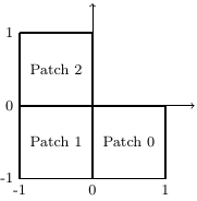
We consider the Laplace problem on an L-shaped domain \( (-1,1)^2 \setminus [0,1]^2 \) which is represented by three squares.

L-shaped domain, 3 patches.

We solve the Laplace problem

\[ -\Delta u = 0~\mathrm{in}~\Omega,\quad u = u_{ex} ~\mathrm{on}~\partial \Omega, \]

where the exact solution \(u_{ex}\) is given in polar coordinates by

\[ u_{ex}(r,\varphi) = r^{\frac{2}{3}} \sin\Big( ( 2\varphi - \pi)/3 \Big). \]

We define exact solution (in Cartesian coordinates) and the (homogenous) right-hand-side of the PDE:

   // Define exact solution (will be used for specifying Dirichlet boundary conditions
   gsFunctionExpr<> g("if( y>0, ( (x^2+y^2)^(1.0/3.0) )*sin( (2*atan2(y,x) - pi)/3.0 ), ( (x^2+y^2)^(1.0/3.0) )*sin( (2*atan2(y,x)+3*pi)/3.0 ) )", 2);
   // Define source function
   gsFunctionExpr<> f("0",2);

Getting geometry and basis

The gsMultiPatch object describing the geometry is read in from an .xml-file:

   // Read xml and create gsMultiPatch
   std::string fileSrc( "planar/lshape2d_3patches_thb.xml" );
   gsMultiPatch<real_t> patches;
   gsReadFile<real_t>( fileSrc, patches);

The information on patch-interfaces and/or boundaries is not necessarily contained in the .xml-file. To make sure that interfaces and boundaries are correctly set up, call gsMultiPatch::computeTopology().

   // Get all interfaces and boundaries:
   patches.computeTopology();

To prescribe Dirichlet boundary conditions on all boundaries, we use the gsMultiPatch::const_biterator to iterate through all boundaries:

   gsBoundaryConditions<> bcInfo;

   // For simplicity, set Dirichlet boundary conditions
   // given by exact solution g on all boundaries:
   for ( gsMultiPatch<>::const_biterator
            bit = patches.bBegin(); bit != patches.bEnd(); ++bit)
   {
       bcInfo.addCondition( *bit, condition_type::dirichlet, &g );
   }

Obtaining the gsMultiBasis from the gsMultiPatch is straightforward, just call the corresponding constructor:

   // Copy basis from the geometry
   gsMultiBasis<> bases( patches );

Note that the resulting gsMultiBasis will be composed of the bases defining the geometry. In this example, the geometry is given as a gsTHBSpline. Accordingly, the created gsMultiBasis is composed of gsTHBSplineBasis.

Get a gsTHBSplineBasis from a gsTensorBSpline

If the geometry is not given as a gsTHBSpline, but as a gsTensorBSpline...

   std::string fileSrcTens( "planar/lshape2d_3patches_tens.xml" );
   gsMultiPatch<real_t> patchesTens;
   gsReadFile<real_t>( fileSrcTens, patchesTens);
   patchesTens.computeTopology();

...one can create a gsTHBSplineBasis as follows:

   // Copy tensor basis
   gsMultiBasis<real_t> basesTens( patchesTens );

   // Create a "basisContainer"
   std::vector< gsBasis<real_t>* > basisContainer;

   // fill the "basisContainer" with patch-wise...
   for ( size_t i = 0; i < basesTens.nBases(); i++)
       basisContainer.push_back(new gsTHBSplineBasis<2,real_t>( basesTens.basis(i) ));

   // finally, create the gsMultiBasis containing gsTHBSpline ...
   gsMultiBasis<real_t> basesFromTens( basisContainer, patches );

Loop

Instead of just solving the problem once, we wrap a loop around the solving process. For each computed solution, we compute the distribution of the error. Based on this error indication, we mark a certain number of cells for refinement.

Setting up adaptive refinement parameters

For adaptive refinement, we need to specify a criterion for marking cells, and a parameter. Currently implemented are PUCA, GARU, errorFraction (a.k.a. Doerfel-marking), see gsMarkElementsForRef().
Setting the parameter to 0 will result in global refinement, setting it to 1 will result in (almost) no refinement.

   // Specify cell-marking strategy...
   MarkingStrategy adaptRefCrit = PUCA;
   //MarkingStrategy adaptRefCrit = GARU;
   //MarkingStrategy adaptRefCrit = errorFraction;

   // ... and parameter.
   const real_t adaptRefParam = 0.9;

Solving the problem

If desired or necessary (e.g., because the geometry is given by a very coarse representation), apply initial uniform (i.e., global) refinement steps:

   // Number of initial uniform refinement steps:
   int numInitUniformRefine  = 2;

   for (int i = 0; i < numInitUniformRefine; ++i)
     bases.uniformRefine();

Wrap a loop around the solution process

   for( int refLoop = 0; refLoop <= numRefinementLoops; refLoop++)
   {

The part re solving the equation is the same as in poisson_example.cpp.

       // Construct assembler
       gsPoissonAssembler<real_t> PoissonAssembler(patches,bases,bcInfo,f);
       PoissonAssembler.options().setInt("DirichletValues", dirichlet::l2Projection);

       // Generate system matrix and load vector
       PoissonAssembler.assemble();

       // Initialize the conjugate gradient solver
       gsSparseSolver<>::CGDiagonal solver( PoissonAssembler.matrix() );

       // Solve the linear system
       gsMatrix<> solVector = solver.solve( PoissonAssembler.rhs() );

       // Construct the isogeometric solution
       gsMultiPatch<> sol;
       PoissonAssembler.constructSolution(solVector, sol);
       // Associate the solution to the patches (isogeometric field)
       gsField<> solField(patches, sol);

Adaptive refinement

After having computed the solution, we compute the local errors. Either by some a posteriori error estimation technique, or, as in this academic example, by computation of the exact error.

       // Compute the error in the H1-seminorm ( = energy norm in this example )
       // using the known exact solution.
       gsExprEvaluator<> ev;
       ev.setIntegrationElements(PoissonAssembler.multiBasis());
       gsExprEvaluator<>::geometryMap Gm = ev.getMap(patches);
       gsExprEvaluator<>::variable is = ev.getVariable(sol);
       auto ms = ev.getVariable(g, Gm);

       // Get the element-wise norms.
       ev.integralElWise( ( igrad(is,Gm) - igrad(ms)).sqNorm()*meas(Gm) );
       const std::vector<real_t> & eltErrs = ev.elementwise();

Having computed the element-wise errors, we select those that need to be marked by calling gsMarkElementsForRef(), where the previously defined parameters adaptRefCrit and adaptRefParam are used. The actual refinement is done by gsRefineMarkedElements().

       // Mark elements for refinement, based on the computed local errors and
       // the refinement-criterion and -parameter.
       std::vector<bool> elMarked;
       gsMarkElementsForRef( eltErrs, adaptRefCrit, adaptRefParam, elMarked);
       for (size_t k=0; k!=elMarked.size(); k++)  gsInfo<<" "<<elMarked[k];
       gsInfo<<"\n";

       // Refine the marked elements with a 1-ring of cells around marked elements
       gsRefineMarkedElements( bases, elMarked, 1 );

       // std::vector<bool> elCMarked;
       // for (size_t k=0; k!=eltErrs.size(); k++) eltErrs[k] = -eltErrs[k];
       //gsMarkElementsForRef( eltErrs, adaptRefCrit, adaptRefParam, elCMarked);
       //gsUnrefineMarkedElements( bases, elCMarked, 1 );

Note/Warning:
As of now, we cannot access a single element of a gsHTensorBasis directly (e.g., by some index). gsMarkElementsForRef() and gsRefineMarkedElements() rely on the assumption that the gsDomainIterator used in these two functions will iterate over the elements in the same order.
This is also the reason why elMarked is a vector of booleans indicating "refine!" or "don't refine!" for each element (instead of, e.g., a list of inidces of elements).

Recall from thbSplineBasis_example.cpp that the refined area must contain the support of at least one basis function. Due to this, we also refine the 1-ring of cells around marked cells.

Adaptive refinement on a gsMultiPatch geometry can result in interfaces which are no longer fully matching. Thus, it is important to call gsMultiBasis::repairInterfaces().

       // Call repair interfaces to make sure that the new meshes
       // match along patch interfaces.
       bases.repairInterfaces( patches.interfaces() );

Plotting final solution

In the last iteration, we export the solution to paraview files

       // Export the final solution
       if( plot && refLoop == numRefinementLoops )
       {
           // Write the computed solution to paraview files
           gsWriteParaview<>(solField, "adaptRef", 1000, true);
       }

Plot the solution in Paraview

   if( plot )
   {
       // Run paraview
       gsFileManager::open("adaptRef.pvd");
   }

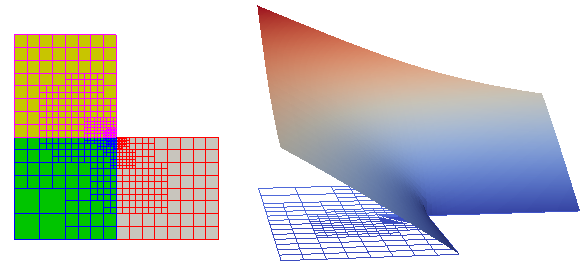
Mesh (left, coloured by patch-index) and solution after 4 adaptive refinement steps.

Annotated source file

Here is the full file examples/adaptRefinementThb_example.cpp. Clicking on a function or class name will lead you to its reference documentation.

# include <gismo.h>
# include <gsAssembler/gsAdaptiveRefUtils.h>

using namespace gismo;

int main(int argc, char *argv[])
{
   bool plot = false;

   // Number of refinement loops to be done
   index_t numRefinementLoops = 4;

   gsCmdLine cmd("Tutorial on solving a Poisson problem.");
   cmd.addSwitch("plot", "Create a ParaView visualization file with the solution", plot);
   cmd.addInt("r", "numLoop", "number of refinement loops", numRefinementLoops);
   try { cmd.getValues(argc,argv); } catch (int rv) { return rv; }

   // --------------- specify exact solution and right-hand-side ---------------

   // Define exact solution (will be used for specifying Dirichlet boundary conditions
   gsFunctionExpr<> g("if( y>0, ( (x^2+y^2)^(1.0/3.0) )*sin( (2*atan2(y,x) - pi)/3.0 ), ( (x^2+y^2)^(1.0/3.0) )*sin( (2*atan2(y,x)+3*pi)/3.0 ) )", 2);
   // Define source function
   gsFunctionExpr<> f("0",2);

   // Print out source function and solution
   gsInfo<<"Source function " << f << "\n";
   gsInfo<<"Exact solution "  << g << "\n\n";


   // --------------- read geometry from file ---------------

   // Read xml and create gsMultiPatch
   std::string fileSrc( "planar/lshape2d_3patches_thb.xml" );
   gsMultiPatch<real_t> patches;
   gsReadFile<real_t>( fileSrc, patches);
   gsInfo << "The domain is a "<< patches <<"\n";

   // Get all interfaces and boundaries:
   patches.computeTopology();


   std::string fileSrcTens( "planar/lshape2d_3patches_tens.xml" );
   gsMultiPatch<real_t> patchesTens;
   gsReadFile<real_t>( fileSrcTens, patchesTens);
   patchesTens.computeTopology();


   // --------------- add bonudary conditions ---------------
   gsBoundaryConditions<> bcInfo;

   // For simplicity, set Dirichlet boundary conditions
   // given by exact solution g on all boundaries:
   for ( gsMultiPatch<>::const_biterator
            bit = patches.bBegin(); bit != patches.bEnd(); ++bit)
   {
       bcInfo.addCondition( *bit, condition_type::dirichlet, &g );
   }


   // --------------- set up basis ---------------

   // Copy basis from the geometry
   gsMultiBasis<> bases( patches );

   // Copy tensor basis
   gsMultiBasis<real_t> basesTens( patchesTens );

   // Create a "basisContainer"
   std::vector< gsBasis<real_t>* > basisContainer;

   // fill the "basisContainer" with patch-wise...
   for ( size_t i = 0; i < basesTens.nBases(); i++)
       basisContainer.push_back(new gsTHBSplineBasis<2,real_t>( basesTens.basis(i) ));

   // finally, create the gsMultiBasis containing gsTHBSpline ...
   gsMultiBasis<real_t> basesFromTens( basisContainer, patches );


   // Number of initial uniform refinement steps:
   int numInitUniformRefine  = 2;

   for (int i = 0; i < numInitUniformRefine; ++i)
     bases.uniformRefine();


   // --------------- set up adaptive refinement loop ---------------



   // Specify cell-marking strategy...
   MarkingStrategy adaptRefCrit = PUCA;
   //MarkingStrategy adaptRefCrit = GARU;
   //MarkingStrategy adaptRefCrit = errorFraction;

   // ... and parameter.
   const real_t adaptRefParam = 0.9;


   // --------------- adaptive refinement loop ---------------

   for( int refLoop = 0; refLoop <= numRefinementLoops; refLoop++)
   {

       // --------------- solving ---------------

       // Construct assembler
       gsPoissonAssembler<real_t> PoissonAssembler(patches,bases,bcInfo,f);
       PoissonAssembler.options().setInt("DirichletValues", dirichlet::l2Projection);

       // Generate system matrix and load vector
       PoissonAssembler.assemble();

       // Initialize the conjugate gradient solver
       gsSparseSolver<>::CGDiagonal solver( PoissonAssembler.matrix() );

       // Solve the linear system
       gsMatrix<> solVector = solver.solve( PoissonAssembler.rhs() );

       // Construct the isogeometric solution
       gsMultiPatch<> sol;
       PoissonAssembler.constructSolution(solVector, sol);
       // Associate the solution to the patches (isogeometric field)
       gsField<> solField(patches, sol);

       // --------------- error estimation/computation ---------------

       // Compute the error in the H1-seminorm ( = energy norm in this example )
       // using the known exact solution.
       gsExprEvaluator<> ev;
       ev.setIntegrationElements(PoissonAssembler.multiBasis());
       gsExprEvaluator<>::geometryMap Gm = ev.getMap(patches);
       gsExprEvaluator<>::variable is = ev.getVariable(sol);
       auto ms = ev.getVariable(g, Gm);

       // Get the element-wise norms.
       ev.integralElWise( ( igrad(is,Gm) - igrad(ms)).sqNorm()*meas(Gm) );
       const std::vector<real_t> & eltErrs = ev.elementwise();

       // --------------- adaptive refinement ---------------

       // Mark elements for refinement, based on the computed local errors and
       // the refinement-criterion and -parameter.
       std::vector<bool> elMarked;
       gsMarkElementsForRef( eltErrs, adaptRefCrit, adaptRefParam, elMarked);
       for (size_t k=0; k!=elMarked.size(); k++)  gsInfo<<" "<<elMarked[k];
       gsInfo<<"\n";

       // Refine the marked elements with a 1-ring of cells around marked elements
       gsRefineMarkedElements( bases, elMarked, 1 );

       // std::vector<bool> elCMarked;
       // for (size_t k=0; k!=eltErrs.size(); k++) eltErrs[k] = -eltErrs[k];
       //gsMarkElementsForRef( eltErrs, adaptRefCrit, adaptRefParam, elCMarked);
       //gsUnrefineMarkedElements( bases, elCMarked, 1 );



       // Call repair interfaces to make sure that the new meshes
       // match along patch interfaces.
       bases.repairInterfaces( patches.interfaces() );


       // Export the final solution
       if( plot && refLoop == numRefinementLoops )
       {
           // Write the computed solution to paraview files
           gsWriteParaview<>(solField, "adaptRef", 1000, true);
       }

   }

   if( plot )
   {
       // Run paraview
       gsFileManager::open("adaptRef.pvd");
   }
   else
   {
       gsInfo<<"Done. No output created, re-run with --plot to get a ParaView "
               "file containing Plotting image data.\n";
   }

   return EXIT_SUCCESS;

}// end main